By Eric Sun (z9sun@ucsd.edu) & Sunan Xu (sux002@ucsd.edu)
Introduction
Abstract
Power outages in the United States can have significant impacts on individuals, communities, businesses, and critical infrastructure. They occur when the supply of electricity to an area is disrupted, resulting in a loss of power. Power outages can occur due to a variety of reasons, including natural disasters, equipment failures, human errors, and intentional acts.
Natural disasters, such as hurricanes, tornadoes, severe storms, earthquakes, and wildfires, can damage power infrastructure, including power lines, transformers, and substations, leading to widespread outages. These events can cause significant disruptions to daily life, including the loss of heating, cooling, lighting, and essential services like healthcare and communication.
Equipment failures, such as malfunctioning transformers, faulty wiring, or aging infrastructure, can also result in power outages. These failures can occur due to regular wear and tear, inadequate maintenance, or unforeseen circumstances.
Human errors, such as construction accidents, excavation damage, or operational mistakes, can inadvertently cause power outages. Additionally, intentional acts of vandalism, sabotage, or cyberattacks targeting the power grid can disrupt the supply of electricity and have severe consequences.
The impacts of power outages can be wide-ranging. They can lead to financial losses for businesses, disrupt critical infrastructure like hospitals and transportation systems, affect communication networks, and compromise public safety. Power outages can also pose risks to vulnerable populations, including the elderly, individuals with medical conditions, and those relying on powered medical devices.
Efforts to minimize power outages and enhance grid resilience involve investments in infrastructure upgrades, regular maintenance, improved monitoring and detection systems, and implementing smart grid technologies. These measures aim to reduce the frequency and duration of outages, enhance response and restoration capabilities, and improve the overall reliability of the power supply.
Understanding the causes and durations of power outages is crucial for developing effective mitigation strategies, improving emergency preparedness, and ensuring a reliable and resilient power grid. By analyzing historical data and identifying patterns and trends, stakeholders can work towards minimizing the impact of power outages and enhancing the overall resilience of the U.S. electrical infrastructure.
Dataset
Throughout this report, we will use the dataset from Purdue University with the name of Major Power Outage Risks in the U.S., which can also be found here. This dataset has major power outage data in the continental U.S. from January 2000 to July 2016.
The dataset provides information on major power outages in the continental United States. It includes details such as the year, month, U.S. state, postal code, NERC (North American Electric Reliability Corporation) region, climate region, cause category, outage duration, electricity demand loss, customers affected, and various economic and demographic characteristics of the affected states.
Number of Rows in the Dataset: 1534 rows.
Question Identification
As a result, we are able to trigger our research question: How do demographic factors of West Coast states influence the duration and affecting range of power outages, and what mitigation strategies can be employed to reduce the risk of outages in these regions?
Some relevant columns:
YEAR: The year when the outage occurred (integer).MONTH: The month when the outage occurred (float).U.S._STATE: The name of the U.S. state where the outage occurred (string).POSTAL.CODE: The postal code of the affected area (string).NERC.REGION: The NERC region where the outage occurred (string).CLIMATE.REGION: The climate region of the affected area (string).CAUSE.CATEGORY: The category of the cause of the outage (string).CAUSE.CATEGORY.DETAIL: Further details about the cause of the outage (string).OUTAGE.DURATION(mins): The duration of the outage in minutes (float).CUSTOMERS.AFFECTED: The number of customers affected by the outage (float).RES.PRICE(cents / kilowatt-hour): Residential price of electricity in cents per kilowatt-hour (float).POPULATION: The population of the state (float).OUTAGE.START: The date and time when the outage started (datetime).OUTAGE.RESTORATION: The date and time when power was restored after the outage (datetime).
Cleaning and EDA (Exploratory Data Analysis)
Data Cleaning
First of all, after downloading the dataset from website, we found it with the format of .xlsx. As a result, we install the openpyxl library and convert it into .csv.
After reading the csv file as a panda dataframe, all the columns are named Unnamed: X. We realized that it was the header information contained in the raw file and the actual data started from the fifth line.
| Major power outage events in the continental U.S. | Unnamed: 1 | Unnamed: 2 | Unnamed: 3 | Unnamed: 4 | Unnamed: 5 | Unnamed: 6 | Unnamed: 7 | Unnamed: 8 | Unnamed: 9 | Unnamed: 10 | Unnamed: 11 | Unnamed: 12 | Unnamed: 13 | Unnamed: 14 | Unnamed: 15 | Unnamed: 16 | Unnamed: 17 | Unnamed: 18 | Unnamed: 19 | Unnamed: 20 | Unnamed: 21 | Unnamed: 22 | Unnamed: 23 | Unnamed: 24 | Unnamed: 25 | Unnamed: 26 | Unnamed: 27 | Unnamed: 28 | Unnamed: 29 | Unnamed: 30 | Unnamed: 31 | Unnamed: 32 | Unnamed: 33 | Unnamed: 34 | Unnamed: 35 | Unnamed: 36 | Unnamed: 37 | Unnamed: 38 | Unnamed: 39 | Unnamed: 40 | Unnamed: 41 | Unnamed: 42 | Unnamed: 43 | Unnamed: 44 | Unnamed: 45 | Unnamed: 46 | Unnamed: 47 | Unnamed: 48 | Unnamed: 49 | Unnamed: 50 | Unnamed: 51 | Unnamed: 52 | Unnamed: 53 | Unnamed: 54 | Unnamed: 55 | Unnamed: 56 | |
|---|---|---|---|---|---|---|---|---|---|---|---|---|---|---|---|---|---|---|---|---|---|---|---|---|---|---|---|---|---|---|---|---|---|---|---|---|---|---|---|---|---|---|---|---|---|---|---|---|---|---|---|---|---|---|---|---|---|
| 0 | Time period: January 2000 - July 2016 | nan | nan | nan | nan | nan | nan | nan | nan | nan | nan | nan | nan | nan | nan | nan | nan | nan | nan | nan | nan | nan | nan | nan | nan | nan | nan | nan | nan | nan | nan | nan | nan | nan | nan | nan | nan | nan | nan | nan | nan | nan | nan | nan | nan | nan | nan | nan | nan | nan | nan | nan | nan | nan | nan | nan | nan |
| 1 | Regions affected: Outages reported in this data file affected a single U.S. state at the time of occurrence | nan | nan | nan | nan | nan | nan | nan | nan | nan | nan | nan | nan | nan | nan | nan | nan | nan | nan | nan | nan | nan | nan | nan | nan | nan | nan | nan | nan | nan | nan | nan | nan | nan | nan | nan | nan | nan | nan | nan | nan | nan | nan | nan | nan | nan | nan | nan | nan | nan | nan | nan | nan | nan | nan | nan | nan |
| 2 | nan | nan | nan | nan | nan | nan | nan | nan | nan | nan | nan | nan | nan | nan | nan | nan | nan | nan | nan | nan | nan | nan | nan | nan | nan | nan | nan | nan | nan | nan | nan | nan | nan | nan | nan | nan | nan | nan | nan | nan | nan | nan | nan | nan | nan | nan | nan | nan | nan | nan | nan | nan | nan | nan | nan | nan | nan |
| 3 | nan | nan | nan | nan | nan | nan | nan | nan | nan | nan | nan | nan | nan | nan | nan | nan | nan | nan | nan | nan | nan | nan | nan | nan | nan | nan | nan | nan | nan | nan | nan | nan | nan | nan | nan | nan | nan | nan | nan | nan | nan | nan | nan | nan | nan | nan | nan | nan | nan | nan | nan | nan | nan | nan | nan | nan | nan |
| 4 | variables | OBS | YEAR | MONTH | U.S._STATE | POSTAL.CODE | NERC.REGION | CLIMATE.REGION | ANOMALY.LEVEL | CLIMATE.CATEGORY | OUTAGE.START.DATE | OUTAGE.START.TIME | OUTAGE.RESTORATION.DATE | OUTAGE.RESTORATION.TIME | CAUSE.CATEGORY | CAUSE.CATEGORY.DETAIL | HURRICANE.NAMES | OUTAGE.DURATION | DEMAND.LOSS.MW | CUSTOMERS.AFFECTED | RES.PRICE | COM.PRICE | IND.PRICE | TOTAL.PRICE | RES.SALES | COM.SALES | IND.SALES | TOTAL.SALES | RES.PERCEN | COM.PERCEN | IND.PERCEN | RES.CUSTOMERS | COM.CUSTOMERS | IND.CUSTOMERS | TOTAL.CUSTOMERS | RES.CUST.PCT | COM.CUST.PCT | IND.CUST.PCT | PC.REALGSP.STATE | PC.REALGSP.USA | PC.REALGSP.REL | PC.REALGSP.CHANGE | UTIL.REALGSP | TOTAL.REALGSP | UTIL.CONTRI | PI.UTIL.OFUSA | POPULATION | POPPCT_URBAN | POPPCT_UC | POPDEN_URBAN | POPDEN_UC | POPDEN_RURAL | AREAPCT_URBAN | AREAPCT_UC | PCT_LAND | PCT_WATER_TOT | PCT_WATER_INLAND |
We then drop the first 4 rows and filter and combine the units line and column names, drop unecessary rows and columns.
| OBS | YEAR | MONTH | U.S._STATE | POSTAL.CODE | NERC.REGION | CLIMATE.REGION | ANOMALY.LEVEL(numeric) | CLIMATE.CATEGORY | OUTAGE.START.DATE(Day of the week, Month Day, Year) | OUTAGE.START.TIME(Hour:Minute:Second (AM / PM)) | OUTAGE.RESTORATION.DATE(Day of the week, Month Day, Year) | OUTAGE.RESTORATION.TIME(Hour:Minute:Second (AM / PM)) | CAUSE.CATEGORY | CAUSE.CATEGORY.DETAIL | HURRICANE.NAMES | OUTAGE.DURATION(mins) | DEMAND.LOSS.MW(Megawatt) | CUSTOMERS.AFFECTED | RES.PRICE(cents / kilowatt-hour) | COM.PRICE(cents / kilowatt-hour) | IND.PRICE(cents / kilowatt-hour) | TOTAL.PRICE(cents / kilowatt-hour) | RES.SALES(Megawatt-hour) | COM.SALES(Megawatt-hour) | IND.SALES(Megawatt-hour) | TOTAL.SALES(Megawatt-hour) | RES.PERCEN(%) | COM.PERCEN(%) | IND.PERCEN(%) | RES.CUSTOMERS | COM.CUSTOMERS | IND.CUSTOMERS | TOTAL.CUSTOMERS | RES.CUST.PCT(%) | COM.CUST.PCT(%) | IND.CUST.PCT(%) | PC.REALGSP.STATE(USD) | PC.REALGSP.USA(USD) | PC.REALGSP.REL(fraction) | PC.REALGSP.CHANGE(%) | UTIL.REALGSP(USD) | TOTAL.REALGSP(USD) | UTIL.CONTRI(%) | PI.UTIL.OFUSA(%) | POPULATION | POPPCT_URBAN(%) | POPPCT_UC(%) | POPDEN_URBAN(persons per square mile) | POPDEN_UC(persons per square mile) | POPDEN_RURAL(persons per square mile) | AREAPCT_URBAN(%) | AREAPCT_UC(%) | PCT_LAND(%) | PCT_WATER_TOT(%) | PCT_WATER_INLAND(%) | |
|---|---|---|---|---|---|---|---|---|---|---|---|---|---|---|---|---|---|---|---|---|---|---|---|---|---|---|---|---|---|---|---|---|---|---|---|---|---|---|---|---|---|---|---|---|---|---|---|---|---|---|---|---|---|---|---|---|
| 0 | 1 | 2011 | 7 | Minnesota | MN | MRO | East North Central | -0.3 | normal | 2011-07-01 00:00:00 | 17:00:00 | 2011-07-03 00:00:00 | 20:00:00 | severe weather | nan | nan | 3060 | nan | 70000 | 11.6 | 9.18 | 6.81 | 9.28 | 2332915 | 2114774 | 2113291 | 6562520 | 35.5491 | 32.225 | 32.2024 | 2.30874e+06 | 276286 | 10673 | 2.5957e+06 | 88.9448 | 10.644 | 0.411181 | 51268 | 47586 | 1.07738 | 1.6 | 4802 | 274182 | 1.75139 | 2.2 | 5.34812e+06 | 73.27 | 15.28 | 2279 | 1700.5 | 18.2 | 2.14 | 0.6 | 91.5927 | 8.40733 | 5.47874 |
| 1 | 2 | 2014 | 5 | Minnesota | MN | MRO | East North Central | -0.1 | normal | 2014-05-11 00:00:00 | 18:38:00 | 2014-05-11 00:00:00 | 18:39:00 | intentional attack | vandalism | nan | 1 | nan | nan | 12.12 | 9.71 | 6.49 | 9.28 | 1586986 | 1807756 | 1887927 | 5284231 | 30.0325 | 34.2104 | 35.7276 | 2.34586e+06 | 284978 | 9898 | 2.64074e+06 | 88.8335 | 10.7916 | 0.37482 | 53499 | 49091 | 1.08979 | 1.9 | 5226 | 291955 | 1.79 | 2.2 | 5.45712e+06 | 73.27 | 15.28 | 2279 | 1700.5 | 18.2 | 2.14 | 0.6 | 91.5927 | 8.40733 | 5.47874 |
| 2 | 3 | 2010 | 10 | Minnesota | MN | MRO | East North Central | -1.5 | cold | 2010-10-26 00:00:00 | 20:00:00 | 2010-10-28 00:00:00 | 22:00:00 | severe weather | heavy wind | nan | 3000 | nan | 70000 | 10.87 | 8.19 | 6.07 | 8.15 | 1467293 | 1801683 | 1951295 | 5222116 | 28.0977 | 34.501 | 37.366 | 2.30029e+06 | 276463 | 10150 | 2.58690e+06 | 88.9206 | 10.687 | 0.392361 | 50447 | 47287 | 1.06683 | 2.7 | 4571 | 267895 | 1.70627 | 2.1 | 5.3109e+06 | 73.27 | 15.28 | 2279 | 1700.5 | 18.2 | 2.14 | 0.6 | 91.5927 | 8.40733 | 5.47874 |
| 3 | 4 | 2012 | 6 | Minnesota | MN | MRO | East North Central | -0.1 | normal | 2012-06-19 00:00:00 | 04:30:00 | 2012-06-20 00:00:00 | 23:00:00 | severe weather | thunderstorm | nan | 2550 | nan | 68200 | 11.79 | 9.25 | 6.71 | 9.19 | 1851519 | 1941174 | 1993026 | 5787064 | 31.9941 | 33.5433 | 34.4393 | 2.31734e+06 | 278466 | 11010 | 2.60681e+06 | 88.8954 | 10.6822 | 0.422355 | 51598 | 48156 | 1.07148 | 0.6 | 5364 | 277627 | 1.93209 | 2.2 | 5.38044e+06 | 73.27 | 15.28 | 2279 | 1700.5 | 18.2 | 2.14 | 0.6 | 91.5927 | 8.40733 | 5.47874 |
| 4 | 5 | 2015 | 7 | Minnesota | MN | MRO | East North Central | 1.2 | warm | 2015-07-18 00:00:00 | 02:00:00 | 2015-07-19 00:00:00 | 07:00:00 | severe weather | nan | nan | 1740 | 250 | 250000 | 13.07 | 10.16 | 7.74 | 10.43 | 2028875 | 2161612 | 1777937 | 5970339 | 33.9826 | 36.2059 | 29.7795 | 2.37467e+06 | 289044 | 9812 | 2.67353e+06 | 88.8216 | 10.8113 | 0.367005 | 54431 | 49844 | 1.09203 | 1.7 | 4873 | 292023 | 1.6687 | 2.2 | 5.48959e+06 | 73.27 | 15.28 | 2279 | 1700.5 | 18.2 | 2.14 | 0.6 | 91.5927 | 8.40733 | 5.47874 |
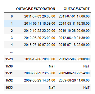
In the data filtering process, we also realize that there are two of each columns related to the start time and restoration time of the power outage in each region. Therefore, we combine OUTAGE.START.DATE and OUTAGE.START.TIME into a new pd.Timestamp column called OUTAGE.START, and combine OUTAGE.RESTORATION.DATE and OUTAGE.RESTORATION.TIME into a new pd.Timestamp column called OUTAGE.RESTORATION, and here are the first few lines of the result columns
After looking at all the column information by use .info(), we found that lots of price, population, or percentage columns that should be in float were all in string data types, and removed the OBS column since the index is the same. Moreover, since all the column names are quite easy to read and understand, so we didn’t change the column names eventually and here is the first several lines of our cleaned dataset:
| YEAR | MONTH | U.S._STATE | POSTAL.CODE | NERC.REGION | CLIMATE.REGION | CLIMATE.CATEGORY | CAUSE.CATEGORY | CAUSE.CATEGORY.DETAIL | HURRICANE.NAMES | OUTAGE.DURATION(mins) | DEMAND.LOSS.MW(Megawatt) | CUSTOMERS.AFFECTED | RES.PRICE(cents / kilowatt-hour) | COM.PRICE(cents / kilowatt-hour) | IND.PRICE(cents / kilowatt-hour) | TOTAL.PRICE(cents / kilowatt-hour) | RES.SALES(Megawatt-hour) | COM.SALES(Megawatt-hour) | IND.SALES(Megawatt-hour) | TOTAL.SALES(Megawatt-hour) | RES.PERCEN(%) | COM.PERCEN(%) | IND.PERCEN(%) | RES.CUSTOMERS | COM.CUSTOMERS | IND.CUSTOMERS | TOTAL.CUSTOMERS | RES.CUST.PCT(%) | COM.CUST.PCT(%) | IND.CUST.PCT(%) | PC.REALGSP.STATE(USD) | PC.REALGSP.USA(USD) | PC.REALGSP.REL(fraction) | PC.REALGSP.CHANGE(%) | UTIL.REALGSP(USD) | TOTAL.REALGSP(USD) | UTIL.CONTRI(%) | PI.UTIL.OFUSA(%) | POPULATION | POPPCT_URBAN(%) | POPPCT_UC(%) | POPDEN_URBAN(persons per square mile) | POPDEN_UC(persons per square mile) | POPDEN_RURAL(persons per square mile) | AREAPCT_URBAN(%) | AREAPCT_UC(%) | PCT_LAND(%) | PCT_WATER_TOT(%) | PCT_WATER_INLAND(%) | OUTAGE.START | OUTAGE.RESTORATION | ANOMALY.LEVEL | |
|---|---|---|---|---|---|---|---|---|---|---|---|---|---|---|---|---|---|---|---|---|---|---|---|---|---|---|---|---|---|---|---|---|---|---|---|---|---|---|---|---|---|---|---|---|---|---|---|---|---|---|---|---|---|
| 0 | 2011 | 7 | Minnesota | MN | MRO | East North Central | normal | severe weather | nan | nan | 3060 | nan | 70000 | 11.6 | 9.18 | 6.81 | 9.28 | 2.33292e+06 | 2.11477e+06 | 2.11329e+06 | 6.56252e+06 | 35.5491 | 32.225 | 32.2024 | 2.30874e+06 | 276286 | 10673 | 2.5957e+06 | 88.9448 | 10.644 | 0.411181 | 51268 | 47586 | 1.07738 | 1.6 | 4802 | 274182 | 1.75139 | 2.2 | 5.34812e+06 | 73.27 | 15.28 | 2279 | 1700.5 | 18.2 | 2.14 | 0.6 | 91.5927 | 8.40733 | 5.47874 | 2011-07-01 17:00:00 | 2011-07-03 20:00:00 | -0.3 |
| 1 | 2014 | 5 | Minnesota | MN | MRO | East North Central | normal | intentional attack | vandalism | nan | 1 | nan | nan | 12.12 | 9.71 | 6.49 | 9.28 | 1.58699e+06 | 1.80776e+06 | 1.88793e+06 | 5.28423e+06 | 30.0325 | 34.2104 | 35.7276 | 2.34586e+06 | 284978 | 9898 | 2.64074e+06 | 88.8335 | 10.7916 | 0.37482 | 53499 | 49091 | 1.08979 | 1.9 | 5226 | 291955 | 1.79 | 2.2 | 5.45712e+06 | 73.27 | 15.28 | 2279 | 1700.5 | 18.2 | 2.14 | 0.6 | 91.5927 | 8.40733 | 5.47874 | 2014-05-11 18:38:00 | 2014-05-11 18:39:00 | -0.1 |
| 2 | 2010 | 10 | Minnesota | MN | MRO | East North Central | cold | severe weather | heavy wind | nan | 3000 | nan | 70000 | 10.87 | 8.19 | 6.07 | 8.15 | 1.46729e+06 | 1.80168e+06 | 1.9513e+06 | 5.22212e+06 | 28.0977 | 34.501 | 37.366 | 2.30029e+06 | 276463 | 10150 | 2.58690e+06 | 88.9206 | 10.687 | 0.392361 | 50447 | 47287 | 1.06683 | 2.7 | 4571 | 267895 | 1.70627 | 2.1 | 5.3109e+06 | 73.27 | 15.28 | 2279 | 1700.5 | 18.2 | 2.14 | 0.6 | 91.5927 | 8.40733 | 5.47874 | 2010-10-26 20:00:00 | 2010-10-28 22:00:00 | -1.5 |
| 3 | 2012 | 6 | Minnesota | MN | MRO | East North Central | normal | severe weather | thunderstorm | nan | 2550 | nan | 68200 | 11.79 | 9.25 | 6.71 | 9.19 | 1.85152e+06 | 1.94117e+06 | 1.99303e+06 | 5.78706e+06 | 31.9941 | 33.5433 | 34.4393 | 2.31734e+06 | 278466 | 11010 | 2.60681e+06 | 88.8954 | 10.6822 | 0.422355 | 51598 | 48156 | 1.07148 | 0.6 | 5364 | 277627 | 1.93209 | 2.2 | 5.38044e+06 | 73.27 | 15.28 | 2279 | 1700.5 | 18.2 | 2.14 | 0.6 | 91.5927 | 8.40733 | 5.47874 | 2012-06-19 04:30:00 | 2012-06-20 23:00:00 | -0.1 |
| 4 | 2015 | 7 | Minnesota | MN | MRO | East North Central | warm | severe weather | nan | nan | 1740 | 250 | 250000 | 13.07 | 10.16 | 7.74 | 10.43 | 2.02888e+06 | 2.16161e+06 | 1.77794e+06 | 5.97034e+06 | 33.9826 | 36.2059 | 29.7795 | 2.37467e+06 | 289044 | 9812 | 2.67353e+06 | 88.8216 | 10.8113 | 0.367005 | 54431 | 49844 | 1.09203 | 1.7 | 4873 | 292023 | 1.6687 | 2.2 | 5.48959e+06 | 73.27 | 15.28 | 2279 | 1700.5 | 18.2 | 2.14 | 0.6 | 91.5927 | 8.40733 | 5.47874 | 2015-07-18 02:00:00 | 2015-07-19 07:00:00 | 1.2 |
Univariate Analysis
The first two plots are based on the column U.S._STATE.
-
The plot titled “State Power Outage Count” is a bar chart that shows the number of power outages for each state. The color of the bars represents the values of the states. By analyzing the plot, we can identify any trends or variations in power outage counts across different states.
Some states have considerably higher outage counts compared to others, indicating a higher frequency of power disruptions. This could be due to various factors such as weather conditions, infrastructure vulnerabilities, or population density. The color encoding provides additional information, potentially highlighting states with particularly severe outage situations.
-
The plot titled “State Frequency Map” is a choropleth map that visualizes the frequency of power outages across different states in the United States. Each state is color-coded based on the number of outages it has experienced. This graph is important as it provides a spatial representation of outage occurrences, allowing us to identify regions with higher outage frequencies and potentially uncover patterns or correlations between geographic factors and outage occurrences.
This visualization helps highlight areas that require closer attention for improving resilience and mitigating power outage risks, which is a more direct visualization comparing to the above bar plot.
The third plot is based on the column CAUSE.CATEGORY.
-
The plot titled “Count of Outages by Cause Category” is a bar chart that displays the number of outages categorized by their cause. Each bar represents a specific cause category, and its height corresponds to the count of outages in that category. This graph is important as it allows us to understand the main causes of power outages and identify the categories that contribute the most to the overall outage count.
The bar chart provides insights into the distribution of power outages based on their cause categories. By analyzing the chart, we can identify the cause categories that are more prevalent in the dataset. This information is valuable for understanding the primary factors leading to power outages and can guide efforts towards implementing preventative measures or improving infrastructure resilience in specific areas.
Bivariate Analysis
-
The plot titled “Residential vs Commercial Sales” is a scatter plot that compares the sales of electricity in megawatt-hours (MWh) for residential and commercial sectors, and the trendline is shown as OLS regression. Each data point represents a state, and its position on the plot indicates the corresponding values for residential and commercial sales. The color of the data points is based on the population of the state. This graph is important as it helps visualize the relationship between residential and commercial electricity sales and identify any potential correlations or trends.
Since we have use
POPULATIONas the color, we can clearly find out the relation that with the increasing population among all regions, the corresponding general sales of electricity will also increment, which again verifies a daily circumstance that we realized every day. -
The plot titled “Outage Duration by Climate Category” is a box plot that displays the distribution of outage durations in minutes across different climate categories. Each box represents a climate category, and the vertical axis represents the duration of outages in minutes. This graph is important as it allows us to compare the outage durations between different climate categories and identify any variations or trends.
-
The plot titled “Correlation Heatmap” visualizes the correlation matrix of the dataset using a color scale. Each cell represents the correlation coefficient between two variables, with cooler colors indicating positive correlations and warmer colors indicating negative correlations. This plot is important as it helps identify relationships and dependencies between different variables in the dataset.
By analyzing the heatmap, we can gain insights into which variables are strongly correlated or inversely correlated, which can guide further analysis and exploration of causal relationships. It can also help identify potential factors that contribute to power outages and inform decision-making for prevention and mitigation strategies.
Interesting Aggregates
- This aggregation named
total_customers_affected_per_yearperformed using thegroupbyfunction calculates the total number of customers affected by power outages each year and presents the results in a pivot table. This table provides a clear overview of the customer impact over time, allowing us to identify trends and patterns in terms of the scale of power outages. The importance of this aggregation lies in understanding the magnitude of the impact on customers and can help prioritize efforts to improve the reliability and resilience of the power grid.
total_customers_affected_per_year = pd.DataFrame(df.groupby('YEAR')['CUSTOMERS.AFFECTED'].sum())
| YEAR | CUSTOMERS.AFFECTED |
|---|---|
| 2000 | 4.27058e+06 |
| 2001 | 1.43141e+06 |
| 2002 | 6.38259e+06 |
| 2003 | 1.24631e+07 |
| 2004 | 1.35926e+07 |
| 2005 | 1.35521e+07 |
| 2006 | 1.01521e+07 |
| 2007 | 5.97343e+06 |
| 2008 | 1.99649e+07 |
| 2009 | 6.81348e+06 |
| 2010 | 1.01081e+07 |
| 2011 | 1.64387e+07 |
| 2012 | 1.2704e+07 |
| 2013 | 7.0184e+06 |
| 2014 | 8.0222e+06 |
| 2015 | 5.62921e+06 |
| 2016 | 1.99391e+06 |
- This pivot table
pivot_table_outage_durationaggregates the average outage duration (in minutes) for each combination of U.S. state and cause category. This table provides insights into the average duration of outages caused by different factors across different states. The importance of this pivot table lies in identifying the causes of longer or more significant outages, which can help prioritize mitigation efforts and improve the reliability of the power grid in specific regions or for specific causes. (The following is the head)
pivot_table_outage_duration = df.pivot_table(index='U.S._STATE', columns='CAUSE.CATEGORY', values='OUTAGE.DURATION(mins)', aggfunc='mean', fill_value=0)
| U.S._STATE | equipment failure | fuel supply emergency | intentional attack | islanding | public appeal | severe weather | system operability disruption |
|---|---|---|---|---|---|---|---|
| Alabama | 0 | 0 | 77 | 0 | 0 | 1421.75 | 0 |
| Arizona | 138.5 | 0 | 639.6 | 0 | 0 | 25726.5 | 384.5 |
| Arkansas | 105 | 0 | 547.833 | 3 | 1063.71 | 2701.8 | 0 |
| California | 524.81 | 6154.6 | 946.458 | 214.857 | 2028.11 | 2928.37 | 363.667 |
| Colorado | 0 | 0 | 117 | 2 | 0 | 2727.25 | 279.75 |
Assessment of Missingness
NMAR
The concept of Not Missing At Random (NMAR) implies that the probability of a value being missing is dependent on the actual missing value itself. In the context of this dataset, the column in question records the names of hurricanes responsible for specific power outages. However, it is important to note that not all power outages can be attributed to hurricanes. Some outages may result from facility maintenance or other natural disasters.
Consequently, if a particular power outage is not caused by a hurricane, it is reasonable for the corresponding cell in the hurricane column to be missing. Incorporating an additional column, such as one that records the amount of rainfall during the corresponding time period, could provide further context. For instance, if the rainfall amount is significantly higher than usual, it is more likely that a hurricane is responsible for the power outage, and thus, the hurricane name column would be shown as NaN. Here is the head of HURRICANE.NAMES column in the dataset:
| HURRICANE.NAMES | |
|---|---|
| 0 | nan |
| 1 | nan |
| 2 | nan |
| 3 | nan |
| 4 | nan |
Missingness Dependency Test 1
In this test, we try to find out if the missingness in CUSTOMERS.AFFECTED column is depend on the the column CAUSE.CATEGORY or not.
| CUSTOMERS.AFFECTED | CAUSE.CATEGORY |
|---|---|
| 70000 | severe weather |
| nan | intentional attack |
| 70000 | severe weather |
| 68200 | severe weather |
| 250000 | severe weather |
| 60000 | severe weather |
| 63000 | severe weather |
| 300000 | severe weather |
| 5941 | intentional attack |
| 400000 | severe weather |
The CUSTOMERS.AFFECTED column signifies the number of individuals impacted by each power outage event, while the CAUSE.CATEGORY column categorizes the specific cause behind these power outages. Prior to commencing our analysis, it is important to examine the patterns and characteristics of the missing data distribution.
The graphical representation of the data reveals a limited number of cause categories, including severe weather and public appeal. Interestingly, a substantial proportion of power outages associated with missing CUSTOMERS.AFFECTED values can be attributed to intentional attack. Conversely, instances where the CUSTOMERS.AFFECTED value is present predominantly align with power outages caused by severe weather. To further ascertain whether the missingness follows a Missing at Random (MAR) pattern, we employ a Total Variation Distance (TVD) test following the permutation of the CUSTOMERS.AFFECTED column. TVD is selected due to the existence of a few cause categories, allowing us to assess the discrepancies between each category for the missing and non-missing groups. A significance level of 0.01 is employed, and the test is iterated 1000 times, yielding the following results:
We get the p-value of 0! , and from the graph we can see that the red line and the distribution of the test result are in the two different world. This disparity strongly indicates that the missingness in the CUSTOMERS.AFFECTED column follows a Missing at Random (MAR) pattern. The evident distinction between the red line and the test result distribution further supports this conclusion. It becomes evident that the CAUSE.CATEGORY column provides valuable insights into the likelihood of missingness within the CUSTOMERS.AFFECTED column.
Missingness Dependency Test 2
In this test, we try to find out if the missingness in CUSTOMERS.AFFECTED column is depend on the the column TOTAL.PRICE or not.
| CUSTOMERS.AFFECTED | TOTAL.PRICE(cents / kilowatt-hour) |
|---|---|
| 70000 | 9.28 |
| nan | 9.28 |
| 70000 | 8.15 |
| 68200 | 9.19 |
| 250000 | 10.43 |
| 60000 | 8.28 |
| 63000 | 9.12 |
| 300000 | 7.36 |
| 5941 | 9.03 |
| 400000 | 10 |
The TOTAL.PRICE column categorizes the overall electricity price for each region which endured the power outage at that time (the unit is cents / kilowatt-hour). Prior to commencing our analysis, lets take a look of data distribution again:
Observing the graphical representation, it becomes apparent that the two graphs exhibit similar patterns. However, in order to further evaluate the comparison between the distribution of the price and its proportion, we employ the Kolmogorov-Smirnov (KS) test statistic following the permutation of the CUSTOMERS.AFFECTED column. The selection of KS is motivated by the desire to assess the similarity of the two groups’ distributions, as they are situated within a similar range on the x-axis. By setting a significance level of 0.01, we iterate the test 1000 times, leading to the following results:
Based on our testing, the obtained p-value is approximately 0.2 (with slight variability upon each code run), surpassing our predetermined significance level. Consequently, we can confidently conclude that there is no significant relationship between the missingness in the CUSTOMERS.AFFECTED column and the TOTAL.PRICE column.
Hypothesis Testing
Hypothesis Testing with column OUTAGE.DURATION
Introduction: Our research question encompasses two main aspects. The first part seeks to understand the influence of demographic factors on the duration of power outages in West states. To investigate this, we focus on two key columns: CLIMATE.REGION and OUTAGE.DURATION.
| OUTAGE.DURATION(mins) | CLIMATE.REGION |
|---|---|
| 3060 | East North Central |
| 1 | East North Central |
| 3000 | East North Central |
| 2550 | East North Central |
| 1740 | East North Central |
| 1860 | East North Central |
| 2970 | East North Central |
| 3960 | East North Central |
| 155 | East North Central |
| 3621 | East North Central |
The CLIMATE.REGION column provides information on the demographic location of each power outage event, while OUTAGE.DURATION indicates the length of time for each outage. Our approach begins by selecting data specifically related to the west climate region. We then employ hypothesis testing to assess whether being located in the West region results in different outage durations compared to the entire nation. By calculating the mean duration of outages in the West region and comparing it to the mean duration of outages across the entire country, we are able to discern notable differences. Specifically, we find that outage durations in the West region are shorter than those experienced nationwide, thereby helping to establish our null and alternative hypotheses.
Null Hypothesis: There is no siginificant difference between outage durations in the West region and those experienced nationwide.
Alternative Hypothesis: Outage durations in the West region are shorter than those experienced nationwide.
Hypothesis test & test statistics : The approach we use is that we will randomly select n rows from teh whole data set, n is the number of outage happened in west region, and calculate the means. Our test statistics is mean of the duration of the random slected rows, and we will compared it with our observed statistic (1628.33 min). The cutoff value is 0.01.
After repeating the test 10000 times, here is what we get:
Our P value is aound (0.0004), we can reject the null hypothesis and conclude that outage durations in the West region are shorter than those experienced nationwide. We are expcted to have a shorter duration of power outage if we are in the west!
Hypothesis Testing with column CUSTOMER.AFFECTED
Introducton: The second part of our research question is to understand the influence of demographic factors on the population affected on each outage. In another words, we are interested at figure out if each outage happened in the west affect more people compared with the the area of the whole country, since it seems like there are lot of people densed aread in the west.
| CLIMATE.REGION | CUSTOMERS.AFFECTED |
|---|---|
| East North Central | 70000 |
| East North Central | nan |
| East North Central | 70000 |
| East North Central | 68200 |
| East North Central | 250000 |
| East North Central | 60000 |
| East North Central | 63000 |
| East North Central | 300000 |
| East North Central | 5941 |
| East North Central | 400000 |
Similar with the previous one, our approach begins by selecting data specifically related to the west climate region. By calculating the number of people affected in the West region and comparing it to the mnumber across the entire country, we are able to discern notable differences.
Null Hypothesis: The number of people affected by power outages on the West region has no siginificant difference with all regions of the country.
Alternative Hypothesis: Compared to the entire country, power outages in the West region affect more people.
Hypothesis test & test statistics : Same as previous one, the approach we use is that we will randomly select n rows from teh whole data set, n is the number of outage happened in west region, and calculate the means of people being affexted. Our test statistics is mean of the population of the random slected rows, and we will compared it with our observed statistic (194579.89). The cutoff value is 0.01.
After repeating the test 10000 times, here is what we get:
Our p-value is aound (0.015), even though it is close, but we can not reject our null hypothesis and can not conclude that the outage happend in the west region affect more people compared with all of the regions in the US.
Conclusion
Overall, as we looked and analyzed through this dataset, we find out that the CLIMATE.REGION with the value of ‘West’ only contains the U.S._STATE of California and Neveda using value_counts(). After analyzing the relationship between columns and hypothesis testing on these two west-region states, we are able to carry out several mitigation strategies:
- California:
-
Enhancing infrastructure resilience: Invest in modernizing and strengthening the power grid infrastructure, including upgrading transmission and distribution systems, implementing smart grid technologies, and enhancing backup power systems.
-
Implementing vegetation management programs: Establish robust vegetation management programs to prevent wildfires caused by contact between vegetation and power lines. Regularly inspect and trim trees near power lines to minimize the risk of outages caused by falling branches or wildfires.
-
Diversifying energy sources: Promote the development and adoption of renewable energy sources such as solar and wind power, along with energy storage solutions. This diversification can reduce reliance on centralized power generation and improve grid stability during extreme weather events.
-
Enhancing communication and coordination: Improve communication and coordination among utility companies, emergency management agencies, and local communities to ensure timely response and efficient restoration efforts during outages. This includes public awareness campaigns, community emergency preparedness initiatives, and clear communication channels.
- Nevada:
-
Implementing grid modernization: Upgrade and modernize the power grid infrastructure, incorporating advanced technologies for monitoring and managing the grid in real-time. This includes deploying sensors, automation systems, and smart meters to detect and respond to outages more efficiently.
-
Strengthening infrastructure against extreme weather: Evaluate and reinforce infrastructure to withstand extreme weather events, such as high winds or heavy snowfall. This includes proactive maintenance of power lines, transformers, and substations to minimize the risk of failures during adverse weather conditions.
-
Enhancing backup power capabilities: Encourage the installation of backup power systems, such as distributed energy resources (DERs) and microgrids, in critical facilities and vulnerable areas. These systems can provide localized power supply during outages, improving resiliency and reducing the impact on essential services.
-
Promoting energy efficiency and demand response: Implement energy efficiency programs to reduce overall energy demand and peak load. Encourage participation in demand response initiatives, where consumers voluntarily reduce electricity usage during periods of high demand, thereby reducing strain on the grid and the likelihood of outages.